Optimisation problem
The equation describes the basic formulation of the optimal power flow (OPF) problem. The pandapower optimal power flow can be constrained by either AC or DC loadflow equations. The branch constraints represent the maximum apparent power loading of transformers and the maximum line current loadings. The bus constraints can contain maximum and minimum voltage magnitude and angle. For the external grid, generators, loads, DC lines and static generators, the maximum and minimum active resp. reactive power can be considered as operational constraints for the optimal power flow. The constraints are defined element wise in the respective element tables.
Generator flexibilities / Operational power constraints
The active and reactive power generation of generators, loads, dc lines and static generators can be defined as a flexibility for the OPF.
Constraint |
Defined in |
\(P_{min,i} \leq P_{g} \leq P_{max,g},\ g \ \epsilon \ gen\) |
net.gen.min_p_mw / net.gen.max_p_mw |
\(Q_{min,g} \leq Q_{g} \leq Q_{max,g},\ g \ \epsilon \ gen\) |
net.gen.min_q_mvar / net.gen.max_q_mvar |
\(P_{min,sg} \leq P_{sg} \leq P_{max,sg},\ sg \ \epsilon \ sgen\) |
net.sgen.min_p_mw / net.sgen.max_p_mw |
\(Q_{min,sg} \leq Q_{sg} \leq Q_{max,sg},\ sg \ \epsilon \ sgen\) |
net.sgen.min_q_mvar / net.sgen.max_q_mvar |
\(P_{max,g},\ g \ \epsilon \ dcline\) |
net.dcline.max_p_mw |
\(Q_{min,g} \leq Q_{g} \leq Q_{max,g},\ g \ \epsilon \ dcline\) |
net.dcline.min_q_from_mvar / net.dcline.max_q_from_mvar / net.dcline.min_q_to_mvar / net.dcline.max_q_to_mvar |
\(P_{min,eg} \leq P_{eg} \leq P_{max,eg},\ eg \ \epsilon \ ext\_grid\) |
net.ext_grid.min_p_mw / net.ext_grid.max_p_mw |
\(Q_{min,eg} \leq Q_{eg} \leq Q_{max,eg},\ eg \ \epsilon \ ext\_grid\) |
net.ext_grid.min_q_mvar / net.ext_grid.max_q_mvar |
\(P_{min,ld} \leq P_{ld} \leq P_{max,ld},\ ld \ \epsilon \ load\) |
net.load.min_p_mw / net.load.max_p_mw |
\(Q_{min,ld} \leq Q_{ld} \leq Q_{max,ld},\ ld \ \epsilon \ load\) |
net.load.min_q_mvar / net.load.max_q_mvar |
\(P_{min,st} \leq P_{st} \leq P_{max,st},\ st \ \epsilon \ storage\) |
net.storage.min_p_mw / net.storage.max_p_mw |
\(Q_{min,st} \leq Q_{st} \leq Q_{max,st},\ st \ \epsilon \ storage\) |
net.storage.min_q_mvar / net.storage.max_q_mvar |
Note
Defining operational constraints is indispensable for the OPF, it will not start if constraints are not defined.
Network constraints
The network constraints contain constraints for bus voltages and branch flows:
Constraint |
Defined in |
\(V_{min,j} \leq V_{g,i} \leq V_{min,i},\ j \ \epsilon \ bus\) |
net.bus.min_vm_pu / net.bus.max_vm_pu |
\(L_{k} \leq L_{max,k},\ k \ \epsilon \ trafo\) |
net.trafo.max_loading_percent |
\(L_{l} \leq L_{max,l},\ l \ \epsilon \ line\) |
net.line.max_loading_percent |
\(L_{l} \leq L_{max,l},\ l \ \epsilon \ trafo_{3w}\) |
net.trafo3w.max_loading_percent |
The defaults are unconstrained branch loadings and \(\pm 1.0 pu\) for bus voltages.
Cost functions
The cost function is specified element wise and is organized in tables as well, which makes the parametrization user friendly. There are two options formulating a cost function for each element: A piecewise linear function with \(n\) data points.
Piecewise linear cost functions can be specified using create_pwl_costs():
- pandapower.create_pwl_cost(net, element, et, points, power_type='p', index=None, check=True, **kwargs)
- Creates an entry for piecewise linear costs for an element. The currently supported elements are
Generator
External Grid
Static Generator
Load
Dcline
Storage
- Parameters:
element (int | integer | Iterable[int | integer]) – ID of the element in the respective element table
et (Literal['gen', 'sgen', 'ext_grid', 'load', 'dcline', 'storage']) – element type, one of “gen”, “sgen”, “ext_grid”, “load”, “dcline”, “storage”
points (list[list[float]]) – list of lists with [[p1, p2, c1], [p2, p3, c2], …] where c(n) defines the costs between p(n) and p(n+1)
power_type (Literal['p', 'q']) – Type of cost [“p”, “q”] are allowed for active or reactive power
index (int | None) – Force a specified ID if it is available. If None, the index one higher than the highest already existing index is selected.
check (bool) – raises UserWarning if costs already exist to this element.
net (pandapowerNet)
- Keyword Arguments:
dataframe (are added as columns to the)
- Returns:
The unique ID of created cost entry
- Raises:
UserWarning – if check is enabled and the element has a cost accociated
- Return type:
int | integer
Example
The cost function is given by the x-values p1 and p2 with the slope m between those points. The constant part b of a linear function y = m*x + b can be neglected for OPF purposes. The intervals have to be continuous (the starting point of an interval has to be equal to the end point of the previous interval).
To create a gen with costs of 1€/MW between 0 and 20 MW and 2€/MW between 20 and 30:
>>> create_pwl_cost(net, 0, "gen", [[0, 20, 1], [20, 30, 2]])
The other option is to formulate a n-polynomial cost function:
Polynomial cost functions can be specified using create_poly_cost():
- pandapower.create_poly_cost(net, element, et, cp1_eur_per_mw, cp0_eur=0., cq1_eur_per_mvar=0., cq0_eur=0., cp2_eur_per_mw2=0., cq2_eur_per_mvar2=0., redispatch_up_eur_per_mw=np.nan, redispatch_down_eur_per_mw=np.nan, index=None, check=True, **kwargs)
- Creates an entry for polynomial costs for an element. The currently supported elements are:
Generator (“gen”)
External Grid (“ext_grid”)
Static Generator (“sgen”)
Load (“load”)
Dcline (“dcline”)
Storage (“storage”)
- Parameters:
element (int | integer | Iterable[int | integer]) – ID of the element in the respective element table
et (Literal['gen', 'sgen', 'ext_grid', 'load', 'dcline', 'storage']) – Type of element [“gen”, “sgen”, “ext_grid”, “load”, “dcline”, “storage”] are possible
cp1_eur_per_mw (float) – Linear costs per MW
cp0_eur (float) – Offset active power costs in euro
cq1_eur_per_mvar (float) – Linear costs per Mvar
cq0_eur (float) – Offset reactive power costs in euro
cp2_eur_per_mw2 (float) – Quadratic costs per MW
cq2_eur_per_mvar2 (float) – Quadratic costs per Mvar
redispatch_up_eur_per_mw (float) – Cost per MW of upward redispatch (increasing active power above the base dispatch). Only used by the redispatch OPF (
runpm_redispatch()). Leave as NaN if the element should not participate in redispatch.redispatch_down_eur_per_mw (float) – Cost per MW of downward redispatch (decreasing active power below the base dispatch). Only used by the redispatch OPF (
runpm_redispatch()). Leave as NaN if the element should not participate in redispatch.index (int | None) – Force a specified ID if it is available. If None, the index one higher than the highest already existing index is selected.
check (bool) – raises UserWarning if costs already exist to this element.
net (pandapowerNet)
- Returns:
The unique ID of created cost entry
- Raises:
UserWarning – if check is enabled and the element has a cost accociated
- Return type:
int | integer
Example
The polynomial cost function is given by the linear and quadratic cost coefficients.
>>> create_poly_cost(net, 0, "load", cp1_eur_per_mw=0.1)
Note
Please note, that polynomial costs for reactive power can only be quadratic, linear or constant. Piecewise linear cost functions for reactive power are not working at the moment with 2 segments or more. Loads can only have 2 data points in their piecewise linear cost function for active power.
Active and reactive power costs are calculated separately. The costs of all types are summed up to determine the overall costs for a grid state.
Visualization of cost functions
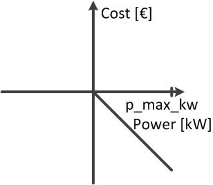
Minimizing generation
The most common optimization goal is the minimization of the overall generator feed in. The according cost function would be formulated like this:
pp.create_poly_cost(net, 0, 'sgen', cp1_eur_per_mw=1)
pp.create_poly_cost(net, 0, 'gen', cp1_eur_per_mw=1)
pp.create_pwl_cost(net, 0, "sgen", [[net.sgen.min_p_mw.at[0], net.sgen.max_p_mw.at[0], 1]])
pp.create_pwl_cost(net, 0, "gen", [[net.gen.min_p_mw.at[0], net.gen.max_p_mw.at[0], 1]])
It is a straight with a negative slope, so that it has the highest cost value at p_min_mw and is zero when the feed in is zero:
Maximizing generation
This cost function may be used, when the curtailment of renewables should be minimized, which at the same time means that the feed in of those renewables should be maximized. This can be realized by the following cost function definitions:
pp.create_poly_cost(net, 0, 'sgen', cp1_eur_per_mw=-1)
pp.create_poly_cost(net, 0, 'gen', cp1_eur_per_mw=-1)
pp.create_pwl_cost(net, 0, "sgen", [[net.sgen.min_p_mw.at[0], net.sgen.max_p_mw.at[0], -1]])
pp.create_pwl_cost(net, 0, "gen", [[net.gen.min_p_mw.at[0], net.gen.max_p_mw.at[0], -1]])
It is a straight with a positive slope, so that the cost is zero at p_min_mw and is at its maximum when the generation equals zero.
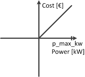
Maximize load
In case that the load should be maximized, the cost function could be defined like this:
pp.create_poly_cost(net, 0, 'load', cp1_eur_per_mw=-1)
pp.create_poly_cost(net, 0, 'storage', cp1_eur_per_mw=-1)
pp.create_pwl_cost(net, 0, "load", [[net.load.min_p_mw.at[0], net.load.max_p_mw.at[0], -1]])
pp.create_pwl_cost(net, 0, "storage", [[net.storage.min_p_mw.at[0], net.storage.max_p_mw.at[0], -1]])
Minimizing load
In case that the load should be minimized, the cost function could be defined like this:
pp.create_poly_cost(net, 0, 'load', cp1_eur_per_mw=1)
pp.create_poly_cost(net, 0, 'storage', cp1_eur_per_mw=1)
pp.create_pwl_cost(net, 0, "load", [[net.load.min_p_mw.at[0], net.load.max_p_mw.at[0], 1]])
pp.create_pwl_cost(net, 0, "storage", [[net.storage.min_p_mw.at[0], net.storage.max_p_mw.at[0], 1]])
DC line behaviour
Please note, that the costs of the DC line transmission are always related to the power at the from_bus!
You can always check your optimization result by comparing your result (From res_sgen, res_load etc.).