Built-in plot functions
In order to get idea about interactive plot features and possibilities see the tutorial.
Simple Plotting
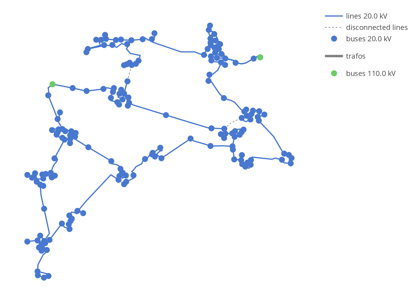
The function simple_plotly() can be used for a simple interactive plotting.
- pandapower.plotting.plotly.simple_plotly(net, respect_switches=True, use_line_geo=None, on_map=False, map_style='basic', figsize=1.0, aspectratio='auto', line_width=1.0, bus_size=10.0, ext_grid_size=20.0, bus_color='blue', line_color='grey', trafo_color='green', trafo3w_color='green', ext_grid_color='yellow', filename='temp-plot.html', auto_open=True, showlegend=True, additional_traces=None, zoomlevel=11, auto_draw_traces=True, hvdc_color='cyan')
Plots a pandapower network as simple as possible in plotly. If no geodata is available, artificial geodata is generated. For advanced plotting see the tutorial
- Parameters:
net (pandapowerNet) – The pandapower format network.
respect_switches (bool, True) – Respect switches when artificial geodata is created
use_line_geo (bool, True) – defines if lines patches are based on net.line.geo of the lines (True) or on net.bus.geo of the connected buses (False)
on_map (bool, False) – enables using mapLibre plot in plotly. If provided geodata are not real geo-coordinates in lon/lat form, on_map will be set to False.
projection (String, None) – defines a projection from which network geo-data will be transformed to lat-long. For each projection a string can be found at http://spatialreference.org/ref/epsg/
map_style (str, 'basic') –
enables using mapLibre plot in plotly
’basic’
’carto-darkmatter’
’carto-darkmatter-nolabels’
’carto-positron’
’carto-positron-nolabels’
’carto-voyager’
’carto-voyager-nolabels’
’dark’
’light’
’open-street-map’
’outdoors’
’satellite’’
’satellite-streets’
’streets’
figsize (float, 1) – aspectratio is multiplied by it in order to get final image size
aspectratio (tuple, 'auto') – when ‘auto’ it preserves original aspect ratio of the network geodata; any custom aspectration can be given as a tuple, e.g. (1.2, 1)
line_width (float, 1.0) – width of lines
bus_size (float, 10.0) – size of buses to plot.
ext_grid_size (float, 20.0) – size of ext_grids to plot. See bus sizes for details. Note: ext_grids are plotted as rectangles
bus_color (String, "blue") – Bus Color. Init as first value of color palette.
line_color (String, 'grey') – Line Color. Init is grey
trafo_color (String, 'green') – Trafo Color. Init is green
trafo3w_color (String, 'green') – Trafo 3W Color. Init is blue
ext_grid_color (String, 'yellow') – External Grid Color. Init is yellow
auto_open (bool, True) – automatically open plot in browser
showlegend (bool, True) – If True, a legend will be shown
additional_traces (list, None) – List with additional, user-created traces that will be appended to the simple_plotly traces before drawing all traces
zoomlevel (int, 11) – initial mapLibre-zoomlevel on a map if on_map=True. Small values = less zoom / larger area shown
auto_draw_traces (bool, True) – if True, a figure with the drawn traces is returned. If False, the traces and a dict with settings is returned
hvdc_color (str, "cyan") – color for HVDC lines
- Returns:
figure object
- Return type:
graph_objs._figure.Figure
Example plot with mv_oberrhein network from the pandapower.networks package:
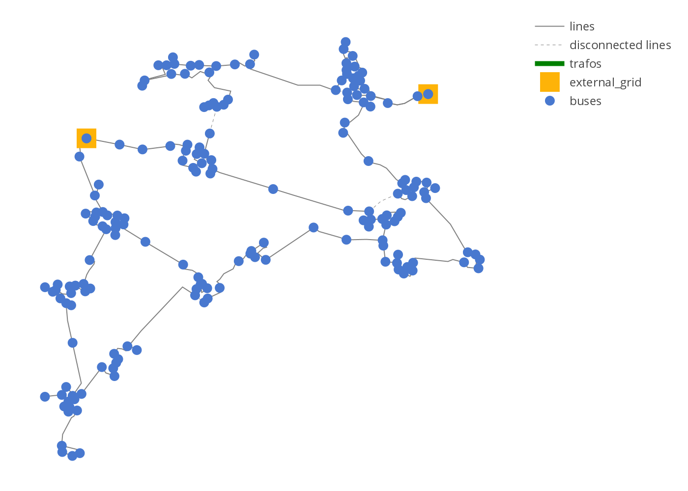
Example simple plot
from pandapower.plotting.plotly import simple_plotly
from pandapower.networks import mv_oberrhein
net = mv_oberrhein()
simple_plotly(net)
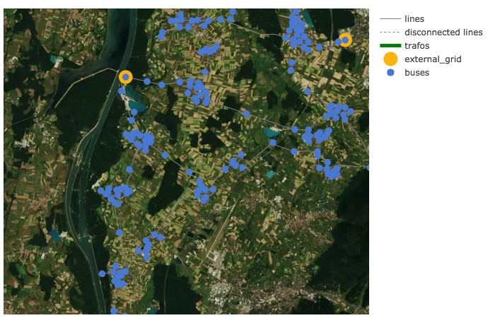
Example simple plot on a map:
net = mv_oberrhein()
simple_plotly(net, on_map=True, projection='epsg:31467')
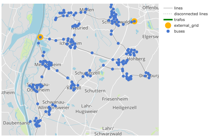
Network coloring according to voltage levels
The function vlevel_plotly() is used to plot a network colored and labeled according to voltage levels.
- pandapower.plotting.plotly.vlevel_plotly(net, respect_switches=True, use_line_geo=None, colors_dict=None, on_map=False, projection=None, map_style='basic', figsize=1, aspectratio='auto', line_width=2, bus_size=10, filename='temp-plot.html', auto_open=True, zoomlevel=11)
Plots a pandapower network in plotly using lines/buses colors according to the voltage level they belong to. If no geodata is available, artificial geodata is generated. For advanced plotting see the tutorial
- Parameters:
net – The pandapower format network.
respect_switches (bool, True) – Respect switches when artificial geodata is created
use_line_geo (bool, True) – defines if lines patches are based on net.line.geo of the lines (True) or on net.bus.geo of the connected buses (False)
colors_dict (dict, None) – dictionary for customization of colors for each voltage level in the form: voltage : color
on_map (bool, False) – enables using mapLibre plot in plotly If provided geodata are not real geo-coordinates in lon/lat form, on_map will be set to False.
projection (String, None) – defines a projection from which network geo-data will be transformed to lat-long. For each projection a string can be found at http://spatialreference.org/ref/epsg/
map_style (str, 'basic') –
enables using mapLibre plot in plotly
’basic’
’carto-darkmatter’
’carto-darkmatter-nolabels’
’carto-positron’
’carto-positron-nolabels’
’carto-voyager’
’carto-voyager-nolabels’
’dark’
’light’
’open-street-map’
’outdoors’
’satellite’’
’satellite-streets’
’streets’
figsize (float, 1) – aspectratio is multiplied by it in order to get final image size
aspectratio (tuple, 'auto') – when ‘auto’ it preserves original aspect ratio of the network geodata any custom aspectration can be given as a tuple, e.g. (1.2, 1)
line_width (float, 1.0) – width of lines
bus_size (float, 10.0) – size of buses to plot.
filename (str, "temp-plot.html") – filename / path to plot to. Should end on *.html
auto_open (bool, True) – automatically open plot in browser
zoomlevel (int, 11) – initial zoomlevel of map plot (only if on_map=True)
- Returns:
figure object
- Return type:
graph_objs._figure.Figure
Example plot with mv_oberrhein network from the pandapower.networks package:
from pandapower.plotting.plotly import vlevel_plotly
from pandapower.networks import mv_oberrhein
net = mv_oberrhein()
vlevel_plotly(net)
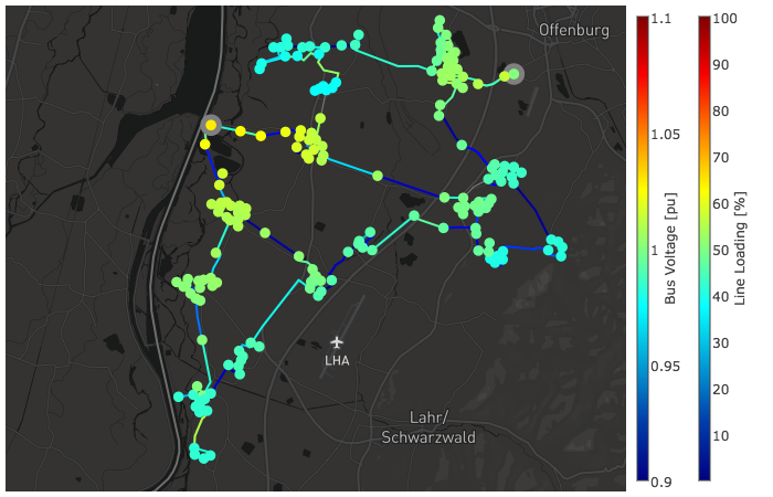
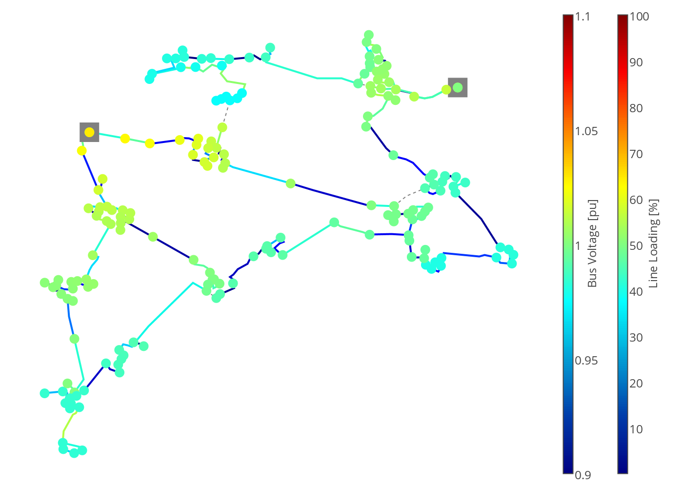
Power Flow results
The function pf_res_plotly() is used to plot a network according to power flow results where a colormap is used to represent line loading and voltage magnitudes. For advanced possibilities see the tutorials.
- pandapower.plotting.plotly.pf_res_plotly(net, cmap='Jet', use_line_geo=None, on_map=False, projection=None, map_style='basic', figsize=1, aspectratio='auto', line_width=2, bus_size=10, climits_volt=(0.9, 1.1), climits_load=(0, 100), cpos_volt=1.0, cpos_load=1.1, filename='temp-plot.html', auto_open=True, zoomlevel=11)
Plots a pandapower network in plotly
using colormap for coloring lines according to line loading and buses according to voltage in p.u. If no geodata is available, artificial geodata is generated. For advanced plotting see the tutorial
- Parameters:
net – The pandapower format network.
respect_switches (bool, False) – Respect switches when artificial geodata is created
cmap (str, True) – name of the colormap
colors_dict (dict, None) – by default 6 basic colors from default collor palette is used. Otherwise, user can define a dictionary in the form: voltage_kv : color
on_map (bool, False) – enables using mapLibre plot in plotly. If provided geodata are not real geo-coordinates in lon/lat form, on_map will be set to False.
projection (String, None) – defines a projection from which network geo-data will be transformed to lat-long. For each projection a string can be found at http://spatialreference.org/ref/epsg/
map_style (str, 'basic') –
enables using mapLibre plot in plotly
’basic’
’carto-darkmatter’
’carto-darkmatter-nolabels’
’carto-positron’
’carto-positron-nolabels’
’carto-voyager’
’carto-voyager-nolabels’
’dark’
’light’
’open-street-map’
’outdoors’
’satellite’’
’satellite-streets’
’streets’
figsize (float, 1) – aspectratio is multiplied by it in order to get final image size
aspectratio (tuple, 'auto') – when ‘auto’ it preserves original aspect ratio of the network geodata any custom aspectration can be given as a tuple, e.g. (1.2, 1)
line_width (float, 1.0) – width of lines
bus_size (float, 10.0) – size of buses to plot.
climits_volt (tuple, (0.9, 1.0)) – limits of the colorbar for voltage
climits_load (tuple, (0, 100)) – limits of the colorbar for line_loading
cpos_volt (float, 1.0) – position of the bus voltage colorbar
cpos_load (float, 1.1) – position of the loading percent colorbar
filename (str, "temp-plot.html") – filename / path to plot to. Should end on *.html
auto_open (bool, True) – automatically open plot in browser
zoomlevel (int, 11) – initial zoomlevel of map plot (only if on_map=True)
- Returns:
figure object
- Return type:
graph_objs._figure.Figure
Example power flow results plot:
from pandapower.plotting.plotly import pf_res_plotly
from pandapower.networks import mv_oberrhein
net = mv_oberrhein()
pf_res_plotly(net)
Power flow results on a map:
net = mv_oberrhein()
pf_res_plotly(net, on_map=True, projection='epsg:31467', map_style='dark')