Built-in plot functions
In order to get idea about interactive plot features and possibilities see the tutorial.
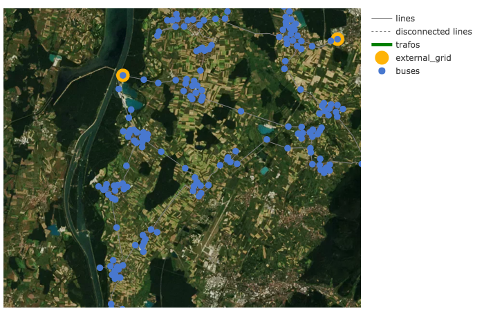
Simple Plotting
The function simple_plotly() can be used for a simple interactive plotting.
- pandapower.plotting.plotly.simple_plotly(net, respect_switches=True, use_line_geo=None, on_map=False, map_style='basic', figsize=1.0, aspectratio='auto', line_width=1.0, bus_size=10.0, ext_grid_size=20.0, bus_color='blue', line_color='grey', trafo_color='green', trafo3w_color='green', ext_grid_color='yellow', filename='temp-plot.html', auto_open=True, showlegend=True, additional_traces=None, zoomlevel=11, auto_draw_traces=True, hvdc_color='cyan')
Plots a pandapower network as simple as possible in plotly. If no geodata is available, artificial geodata is generated. For advanced plotting see the tutorial
- Parameters:
**net** (pandapowerNet)
**respect_switches** (bool, True)
**use_line_geo** (bool, True)
lines (net.line.geo of the)
**on_map** (bool, False)
form (If provided geodata are not real geo-coordinates in lon/lat)
False. (on_map will be set to)
**projection** (String, None)
http (lat-long. For each projection a string can be found at) – //spatialreference.org/ref/epsg/
**map_style** (str, 'basic') –
‘basic’
’carto-darkmatter’
’carto-darkmatter-nolabels’
’carto-positron’
’carto-positron-nolabels’
’carto-voyager’
’carto-voyager-nolabels’
’dark’
’light’
’open-street-map’
’outdoors’
’satellite’’
’satellite-streets’
’streets’
**figsize** (float, 1)
**aspectratio** (tuple, 'auto')
tuple (any custom aspectration can be given as a)
e.g. (1.2, 1)
**line_width** (float, 1.0)
**bus_size** (float, 10.0)
**ext_grid_size** (float, 20.0) – See bus sizes for details. Note: ext_grids are plotted as rectangles
**bus_color** (String, "blue")
**line_color** (String, 'grey')
**trafo_color** (String, 'green')
**trafo3w_color** (String, 'green')
**ext_grid_color** (String, 'yellow')
**auto_open** (bool, True)
**showlegend** (bool, True)
**additional_traces** (list, None)
traces (be appended to the simple_plotly traces before drawing all)
**zoomlevel** (int, 11)
shown (values = less zoom / larger area)
**auto_draw_traces** (bool, True)
False (If)
returned (the traces and a dict with settings is)
**hvdc_color** (str, "cyan")
- Returns:
figure (graph_objs._figure.Figure) figure object
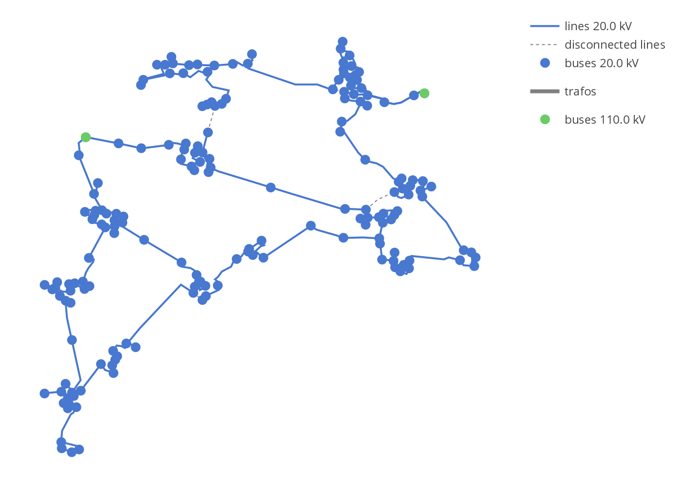
Example plot with mv_oberrhein network from the pandapower.networks package:
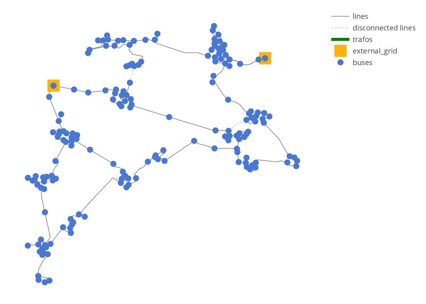
Example simple plot
from pandapower.plotting.plotly import simple_plotly
from pandapower.networks import mv_oberrhein
net = mv_oberrhein()
simple_plotly(net)
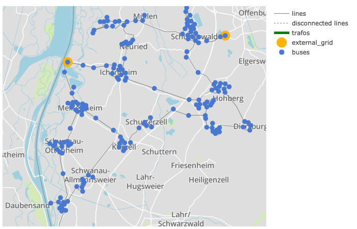
Example simple plot on a map:
net = mv_oberrhein()
simple_plotly(net, on_map=True, projection='epsg:31467')
Network coloring according to voltage levels
The function vlevel_plotly() is used to plot a network colored and labeled according to voltage levels.
- pandapower.plotting.plotly.vlevel_plotly(net, respect_switches=True, use_line_geo=None, colors_dict=None, on_map=False, projection=None, map_style='basic', figsize=1, aspectratio='auto', line_width=2, bus_size=10, filename='temp-plot.html', auto_open=True, zoomlevel=11)
Plots a pandapower network in plotly using lines/buses colors according to the voltage level they belong to. If no geodata is available, artificial geodata is generated. For advanced plotting see the tutorial
- Parameters:
network. (**net** - The pandapower format)
**respect_switches** (bool, True)
**use_line_geo** (bool, True)
lines (of the)
*colors_dict** (dict, None)
form (real geo-coordinates in lon/lat) – voltage : color
**on_map** (bool, False)
form
False. (on_map will be set to)
**projection** (String, None)
at (transformed to lat-long. For each projection a string can be found)
http – //spatialreference.org/ref/epsg/
**map_style** (str, 'basic') –
‘basic’
’carto-darkmatter’
’carto-darkmatter-nolabels’
’carto-positron’
’carto-positron-nolabels’
’carto-voyager’
’carto-voyager-nolabels’
’dark’
’light’
’open-street-map’
’outdoors’
’satellite’’
’satellite-streets’
’streets’
**figsize** (float, 1)
**aspectratio** (tuple, 'auto')
tuple (network geodata any custom aspectration can be given as a)
e.g. (1.2, 1)
**line_width** (float, 1.0)
**bus_size** (float, 10.0)
**filename** (str, "temp-plot.html")
**auto_open** (bool, True)
**zoomlevel** (int, 11) - initial zoomlevel of map plot (only if on_map=True)
- Returns:
figure (graph_objs._figure.Figure) figure object
Example plot with mv_oberrhein network from the pandapower.networks package:
from pandapower.plotting.plotly import vlevel_plotly
from pandapower.networks import mv_oberrhein
net = mv_oberrhein()
vlevel_plotly(net)
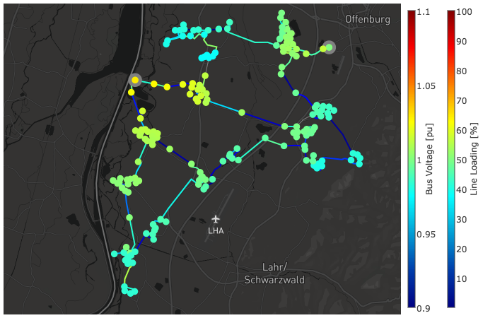
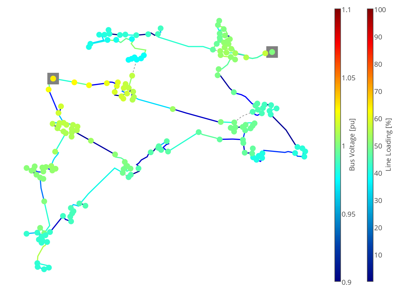
Power Flow results
The function pf_res_plotly() is used to plot a network according to power flow results where a colormap is used to represent line loading and voltage magnitudes. For advanced possibilities see the tutorials.
- pandapower.plotting.plotly.pf_res_plotly(net, cmap='Jet', use_line_geo=None, on_map=False, projection=None, map_style='basic', figsize=1, aspectratio='auto', line_width=2, bus_size=10, climits_volt=(0.9, 1.1), climits_load=(0, 100), cpos_volt=1.0, cpos_load=1.1, filename='temp-plot.html', auto_open=True, zoomlevel=11)
Plots a pandapower network in plotly
using colormap for coloring lines according to line loading and buses according to voltage in p.u. If no geodata is available, artificial geodata is generated. For advanced plotting see the tutorial
- Parameters:
network. (**net** - The pandapower format)
**respect_switches** (bool, False)
**cmap** (str, True)
**colors_dict** (dict, None)
Otherwise – voltage_kv : color
form (real geo-coordinates in lon/lat) – voltage_kv : color
**on_map** (bool, False)
form
False. (on_map will be set to)
**projection** (String, None)
http (lat-long. For each projection a string can be found at) – //spatialreference.org/ref/epsg/
**map_style** (str, 'basic') –
‘basic’
’carto-darkmatter’
’carto-darkmatter-nolabels’
’carto-positron’
’carto-positron-nolabels’
’carto-voyager’
’carto-voyager-nolabels’
’dark’
’light’
’open-street-map’
’outdoors’
’satellite’’
’satellite-streets’
’streets’
**figsize** (float, 1)
**aspectratio** (tuple, 'auto')
tuple (any custom aspectration can be given as a)
e.g. (1.2, 1)
**line_width** (float, 1.0)
**bus_size** (float, 10.0)
**climits_volt** (tuple, (0.9, 1.0))
**climits_load** (tuple, (0, 100))
**cpos_volt** (float, 1.0)
**cpos_load** (float, 1.1)
**filename** (str, "temp-plot.html")
**auto_open** (bool, True)
**zoomlevel** (int, 11) - initial zoomlevel of map plot (only if on_map=True)
- Returns:
figure (graph_objs._figure.Figure) figure object
Example power flow results plot:
from pandapower.plotting.plotly import pf_res_plotly
from pandapower.networks import mv_oberrhein
net = mv_oberrhein()
pf_res_plotly(net)
Power flow results on a map:
net = mv_oberrhein()
pf_res_plotly(net, on_map=True, projection='epsg:31467', map_style='dark')